Getting Started

What is IBM StreamSets for Apache Spark?

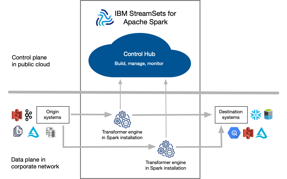
IBM^© StreamSets for Apache Spark is a cloud-native platform for building, running, and monitoring data pipelines on Apache Spark.

A pipeline describes the flow of data from origin systems to destination systems and defines how to process the data along the way. Pipelines can access multiple types of external systems, including cloud data lakes, cloud data warehouses, and storage systems installed on-premises such as relational databases.

As a pipeline runs, you can view real-time statistics and error information about the data as it flows from origin to destination systems.

IBM StreamSets for Apache Spark uses the following components to manage your pipelines:

Control Hub: Control Hub is a fully-managed cloud service that you access using a web browser. Use Control Hub to build, manage, and monitor your pipelines.

Transformer: Transformer is an engine that processes data. Use the engine to run data processing pipelines on Apache Spark. Because Transformer pipelines run on Spark deployed on a cluster, the pipelines can perform set-based transformations such as joins, aggregates, and sorts on the entire data set.; You deploy Transformer engines in your corporate network, which can be on-premises or on a protected cloud computing platform.; When you start a pipeline from Control Hub, the engine launches distributed Spark applications that process the data based on the pipeline configuration. The engine sends status updates and metrics about the running pipeline back to Control Hub so that you can monitor the pipeline progress in real time.

The following image provides a general overview of the IBM StreamSets for Apache Spark components:

Pipeline Processing on Spark

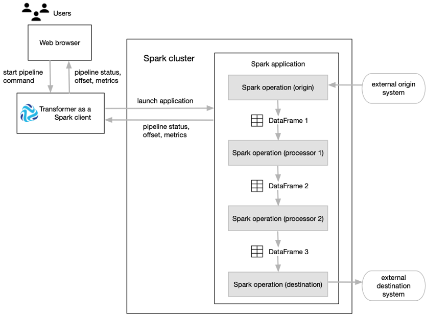
Transformer functions as a Spark client that launches distributed Spark applications.

When you start a pipeline on a Hadoop cluster, Transformer uses the Spark Launcher API to launch a Spark application. When you start a pipeline on a Databricks cluster, Transformer uses the Databricks REST API to run a Databricks job which launches a Spark application.

Transformer passes the pipeline definition in JSON format as an application argument. Spark runs the application just as it runs any other application, distributing the processing across nodes in the cluster.

Note: To get started with Transformer in a development environment, you can simply install both Transformer and Spark on the same machine and run Spark locally on that machine. In this case, Spark runs each application on the single machine.

Each pipeline stage represents a Spark operation:

The Spark operation for an origin reads data from the origin system in a batch. The origin represents the data as a Spark DataFrame and passes the DataFrame to the next operation.
The Spark operation for each processor receives a DataFrame, operates on that data, and then returns a new DataFrame that is passed to the next operation.
The Spark operation for a destination receives a DataFrame, converts the DataFrame to the specified data format such as Avro, Delimited, JSON, or Parquet, and then writes the converted data to the destination system.

As the Spark application runs, you use the Control Hub UI to monitor the progress of the pipeline and troubleshoot any errors. When you stop the pipeline, Transformer stops the Spark application.

The following image shows how Transformer submits a pipeline to Spark as an application and how Spark runs that application:

Batch Case Study

Transformer can run pipelines in batch mode. A batch pipeline processes all available data in a single batch, and then stops.

A batch pipeline is typically used to process data that has already been stored over a period of time, often in a relational database or in a raw or staging area in a Hadoop Distributed File System (HDFS).

Let's say that you have an existing data warehouse in a relational database. You need to create a data mart for the sales team that includes a subset of the data warehouse tables. To create the data mart, you need to join data from the Retail and StoreDetails tables using the store zip code field. The Retail table includes transactional data for each order, including the product ID, unit price, store ID, and store zip code. The StoreDetails table includes demographic data for each store zip code, such as the city and population.

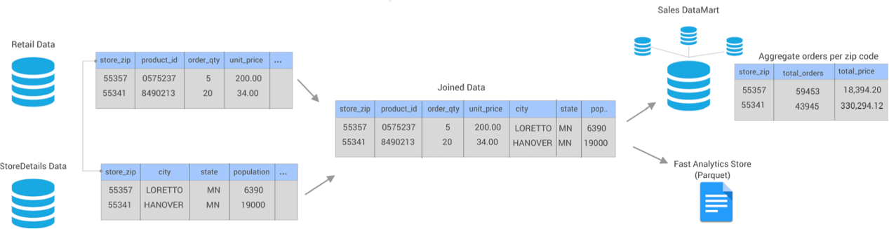
You also need to aggregate the data before sending it to the sales data mart to calculate the total revenue and total number of orders for each zip code.

In addition, you need to send the same joined data from the Retail and StoreDetails tables to Parquet files so that data scientists can efficiently analyze the data. To increase the analytics performance, you need to create a surrogate key for the data and then write the data to a small set of Parquet files.

The following image shows a high-level design of the data flow and some of the sample data:

You can use Transformer to create and run a single batch pipeline to meet all of these needs.

Let's take a closer look at how you design the batch pipeline:

Set execution mode to batch: On the General tab of the pipeline, you set the execution mode to batch.
Join data from two source tables: You add two JDBC Table origins to the pipeline, configuring one to read from the Retail database table and the other to read from the StoreDetails table. You want both origins to read all rows in each table in a single batch, so you use the default value of -1 for the Max Rows per Batch property for the origins.; You add a Join processor to perform an inner join on the data read by the two origins, joining data by the matching store zip code field.; Note that if you prefer to create a custom query that reads from the two tables, you can use a single JDBC Query origin instead of these three stages. However, the JDBC Table origins allow you to read from tables without configuring a query.
Aggregate data before writing to the data mart: You create one pipeline branch that performs the processing needed for the sales data mart.; After the Join processor, you add an Aggregate processor that calculates the total revenue and total number of orders for each zip code.; Finally, you add a JDBC destination to write the transformed data to the data mart.
Create a surrogate key and repartition the data before writing to Parquet files: You create a second pipeline branch to perform the processing needed for the Parquet files used by data scientists.; You add a Surrogate Key Generator processor to generate a unique surrogate key for each record in the input data.; The Join processor causes Spark to shuffle the data, splitting the data into a large number of partitions. However, since this branch writes to Parquet files, the data must be written to a small number of files for data scientists to efficiently analyze the data. So you add a Repartition processor to decrease the number of partitions to four.; Finally, you add a File destination to the branch to write the data to Parquet files. The File destination creates one output file for each partition, so this destination creates a total of four output files.

The following image shows the complete design of this batch pipeline:

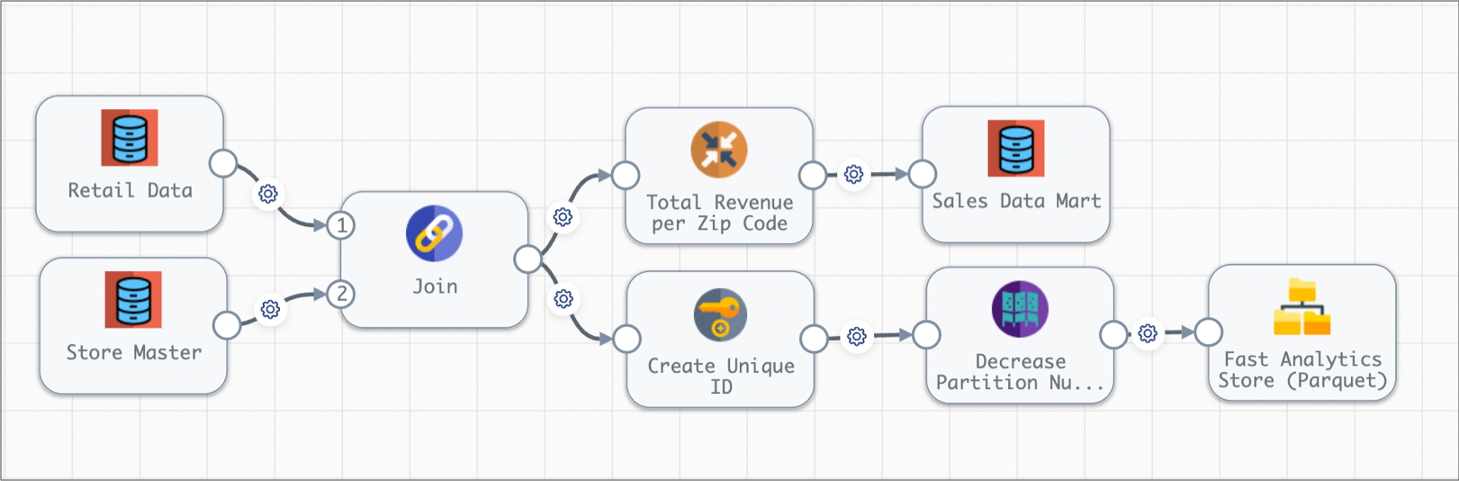
When you start this batch pipeline, the pipeline reads all available data in both database tables in a single batch. Each processor transforms the data, and then each destination writes the data to the data mart or to Parquet files. After processing all the data in a single batch, the pipeline stops.

Streaming Case Study

Transformer can run pipelines in streaming mode. A streaming pipeline maintains connections to origin systems and processes data at user-defined intervals. The pipeline runs continuously until you manually stop it.

A streaming pipeline is typically used to process data in stream processing platforms such as Apache Kafka.

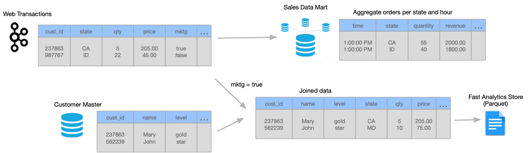
Let's say that your website transactions are continuously being sent to Kafka. The website transaction data includes the customer ID, shipping address, product ID, quantity of items, price, and whether the customer accepted marketing campaigns.

You need to create a data mart for the sales team that includes aggregated data about the online orders, including the total revenue for each state by the hour. Because the transaction data continuously arrives, you need to produce one-hour windows of data before performing the aggregate calculations.

You also need to join the same website transaction data with detailed customer data from your data warehouse for the customers accepting marketing campaigns. You must send this joined customer data to Parquet files so that data scientists can efficiently analyze the data. To increase the analytics performance, you need to write the data to a small set of Parquet files.

The following image shows a high-level design of the data flow and some of the sample data:

You can use Transformer to create and run a single streaming pipeline to meet all of these needs.

Let's take a closer look at how you design the streaming pipeline:

Set execution mode to streaming: On the General tab of the pipeline, you set the execution mode to streaming. You also specify a trigger interval that defines the time that the pipeline waits before processing the next batch of data. Let's say you set the interval to 1000 milliseconds - that's 1 second.
Read from Kafka and then create one-hour windows of data: You add a Kafka origin to the Transformer pipeline, configuring the origin to read from the weborders topic in the Kafka cluster.; To create larger batches of data for more meaningful aggregate calculations, you add a Window processor. You configure the processor to create a tumbling window using one-hour windows of data.
Aggregate data before writing to the data mart: You create one pipeline branch that performs the processing needed for the sales data mart.; You want to aggregate the data by the shipping address state and by the hour. After the Window processor, you add a Spark SQL Expression processor that uses the current_timestamp() Spark SQL function to calculate the current time and write the value to a new time field. Then you add an Aggregate processor that calculates the total revenue and total number of orders by each state and hour.; Finally, you add a JDBC destination to write the transformed data to the data mart.
Filter, join, and repartition the data before writing to Parquet files: You create a second pipeline branch to perform the processing needed for the Parquet files used by data scientists.; You add a Filter processor to pass records downstream where the customer accepted marketing campaigns. The Filter processor drops all records where the customer declined the campaigns.; You add a JDBC Table origin to the pipeline, configuring the origin to read from the Customers database table. You want the origin to read all rows in a single batch, so you use the default value of -1 for the Max Rows per Batch property. You configure the origin to load the data only once so that the origin reads from the table once and then stores the data on the Spark nodes. When processing subsequent batches, the pipeline looks up that data on the Spark nodes.; You add a Join processor to perform an inner join on the data produced by the Filter processor and the data produced by the JDBC Table origin, joining data by the matching customer ID field.; The Join processor causes Spark to shuffle the data, splitting the data into a large number of partitions. However, since this branch writes to Parquet files, the data must be written to a small number of files for data scientists to efficiently analyze the data. So you add a Repartition processor to decrease the number of partitions to four.; Finally, you add a File destination to the branch to write the data to Parquet files. The File destination creates one output file for each partition, so this destination creates a total of four output files.

The following image shows the complete design of this streaming pipeline:

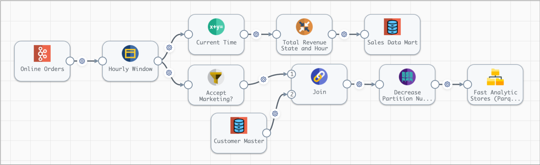
When you start this streaming pipeline, the pipeline reads the available online order data in Kafka. The pipeline reads customer data from the database once, storing the data on the Spark nodes for subsequent lookups.

Each processor transforms the data, and then each destination writes the data to the data mart or to Parquet files. After processing all the data in a single batch, the pipeline waits 1 second, then reads the next batch of data from Kafka and reads the database data stored on the Spark nodes. The pipeline runs continuously until you manually stop it.

Tutorials and Sample Pipelines

StreamSets provides tutorials and sample pipelines to help you learn about using Transformer.

You can find StreamSets tutorials on Github. Transformer also includes several sample pipelines. You can use these pipelines to walk through tutorials or as a basis for new development.